

Theory For FOC Control-2
Preface
In the previous chapter, we introduced the types of motors and briefly described their control methods. In this chapter, we will delve into the mathematical model and FOC control method in depth
Control state

Here you can refer to the dynamic diagram of the left image, where it can be seen that different current directions pass through to generate a magnetic field direction in the stator, causing rotation of the rotor due to the repulsion of opposite poles.
This rotational state can be further subdivided into 6 different states, which will be discussed separately below

The six different current directions in the above figure can be tabulated to obtain the figure below. The position of the rotor in each of the six steps depends on the rotor position, which can usually be sensed by sensors or inferred by back electromotive force (EMF) when the motor is not energized.

The current diagram can be obtained by tabulating the six different current directions in the above figure, and which step the motor is in depends on the position of the rotor, which can be sensed by sensors or calculated by back-EMF when there is no current flowing. Then, to implement the current diagram, a three-phase inverter circuit is used (which corresponds to the motor driver for BLDC)

PS:Please note that the waveform in the above figure may look like the six-step square wave drive for BLDC, but upon closer examination, it can be observed that it is a current waveform instead of voltage.
Three-phase inverter circuit

The VT in the above circuit refers to the IGBT module, and in low-power drive, MOSFET is generally used as a switch. Both are fully controlled devices and can be regarded as high-speed electronic switches controlled by voltage. By applying high or low frequency to the gate of the MOSFET (High Drive and Low Drive in the above figure), the conduction or turn-off of the MOS source and drain can be controlled.
In the figure below, we activate the upper bridge arms of the first group of half-bridges, and the lower bridge arms of the second and third group of half-bridges (the rest are turned off), that is, we turn on VT1, VT2, and VT6. This will allow current to flow from the positive terminal of the power supply through phase a of the motor, then through phases b and c, and then back to the negative terminal of the power supply.

The following figure shows the situation for the upper two arms and lower arm:

By controlling the different switch states of the three half-bridges, we can control the current flow in the motor in different directions.
In this way, at any given moment, three bridge arms will be conducting simultaneously. It could be the upper arm and the two lower arms, or it could be the upper two arms and the lower arm. Because each commutation is carried out between the upper and lower bridge arms of the same phase, it is also known as longitudinal commutation.
Clarke’s Transformation AND Park’s Transformation
Here is a concept first: it is very demanding for components and control methods to directly control the current output as a sine wave. Therefore, is there a way to transform the sine wave into a linear one? This is where the Clarke and Park transformations come in. Two images will help you understand what these two transformations are doing.
Clarke’s Transformation
Clarke’s Transformation simplifies the three-phase waveforms into two rotating waves (this simplification method is simply a coordinate transformation).

Park’s Transformation
Park’s Transformation further transforms the 2 sinusoidal waves into 2 linear lines.

Mathematical formula
First, let’s look at the inertial coordinate system of the motor during rotation.


As shown in the above figure, the direction of the resulting force generated by three different input voltage waveforms can be observed. First, let’s observe the change of the input current in this coordinate system to use it as a feedback signal for control. The first step is the Clarke’s Transformation, which transforms the inertial coordinate system into the orthogonal coordinate system αβ.

As shown in the figure above, the two coordinate systems are overlapped, where N3 is the effective turns of each phase of the abc coordinate three-phase winding, and N2 is the effective turns of each phase of the αβ coordinate winding.
Note that the coordinate transformation must satisfy the following two points:
- The rotating magnetic field generated by the current before and after the transformation must be equivalent.
- The rotating magnetic field generated by the current before and after the transformation should be equivalent” and “The motor power remains unchanged before and after the transformation.


The above formula is equivalently projected onto the αβ coordinate system and written in matrix form as shown on the upper right. However, the above formula cannot be inverted, so a modification is needed by adding another axis 0 (which is mostly not important and can be ignored).

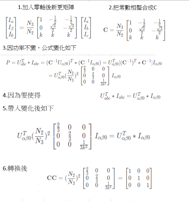
由右邊推導最後可以求得如下
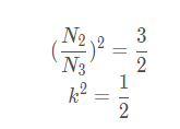
Then the amplitude conversion process is as follows:


Since we need equal amplitude, Ib is in phase with Ia and α leads β by 90 degrees. This can be simplified into the following equation


Summarize
The Clarke transformation formula is as follows:


After understanding the Clarke’s Transformation, the next step is to transform the sinusoidal signals into linear signals using Park’s Transformation.


Here, the Park’s Transformation is simply a straightforward transformation from the inertial coordinate system to a non-inertial coordinate system (a hypothetical coordinate system) to simplify the analysis and reduce it to a linear relationship.

Summarize
