Difference between single-shunt and three-shunt
Preface
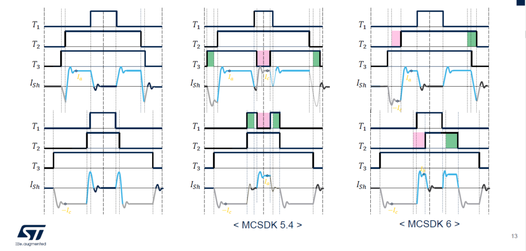
Here, for design reference, a detailed exploration of single-shunt and three-shunt configurations is conducted. This article will delve into the differences between these two configurations and the variances between the old and new versions of MCSDK. It is recommended to use MCSDK 5.x version for verification, as it provides a better UI interface for validation. MCSDK 6.x comes with improved algorithms for the 1-shunt configuration.
Shunt Resistor Design
In the previous section, different shunt resistor designs were mentioned. Here, we will briefly review the system.
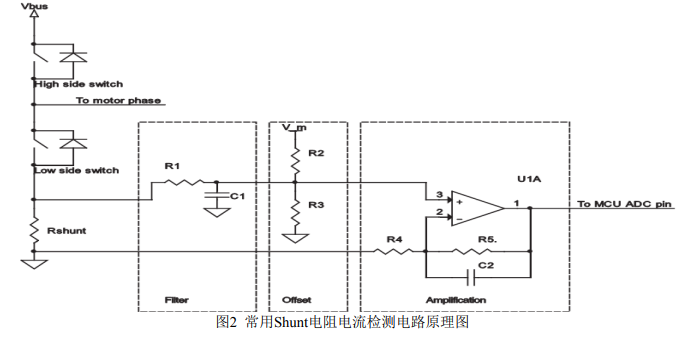
The design is essentially divided into three parts: Filter, Offset, and OPA (Operational Amplifier). The inclusion of a Filter is not mandatory, as adding an RC Filter can slow down the response speed. This may not be favorable in some speed control applications. However, incorporating an RC Filter can improve resistance to rapid deceleration, preventing excessive Overshoot and detection errors.
The Offset part is essential, as ADC cannot receive negative values. Finally, the OPA section depends on the specific requirements and the need for adjusting gain values.
Introduction to 3-Shunt
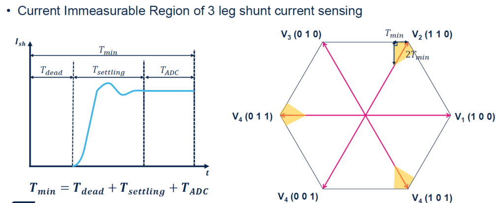
The flexibility of current detection in a 3-shunt configuration is higher. This is due to the formula 𝐼𝑎 + 𝐼𝑏 + 𝐼𝑐 = 0, where selecting any two out of the three shunts allows the calculation of the entire current. Therefore, compared to 1-shunt detection, there is no need for complex algorithms and detection dead zones in 3-shunt configuration. However, the cost of 3-shunt design is higher than that of 1 shunt.

The threeshunt technique can bounce sampling between current signals, selecting two out of three phases each
period, which allows long time periods for the current signals to settle.
However, as with algorithm compensation, there may be areas where calculation is not possible, as seen in the 3-shunt dead zone chart.
Introduction to 1-Shunt
A 1-shunt configuration is generally more complex, primarily due to algorithm compensation. The formula 𝐼𝑎 + 𝐼𝑏 + 𝐼𝑐 = 0 applies in this case.

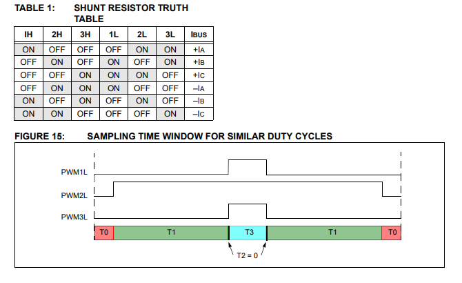
You can also refer to this diagram, which shows the High Side and Low Side sections. It is similar to the previous diagram, as the upper and lower arms do not conduct simultaneously.
“n common motor control applications, the PWM frequency is generally between 10KHz and 20KHz. Taking 20KHz as an example, one PWM cycle is 50us. Within the 50us window, three-phase currents need to be detected, so the detection window for each phase current is 50/3us multiplied by the PWM duty cycle. In motor control systems, the minimum PWM duty cycle is often defined as 5%, so the minimum detection window for each phase current is 50/3us × 5% = 0.83us. In program control, the ADC sampling instant is often controlled to be in the middle of this current detection window. Therefore, for the Shunt current detection circuit, it must stabilize before the ADC sampling instant, completing the establishment of the voltage signal stably.
Assuming the rising edge time occupies 20% of the current detection window, i.e., 20% × 0.83us = 0.167us, then for a 3.3V MCU, the minimum slew rate SR = 3.3V/0.167us = 19.76V/us. At the same time, the bandwidth used should be much greater than the PWM frequency, at least 10 times higher.
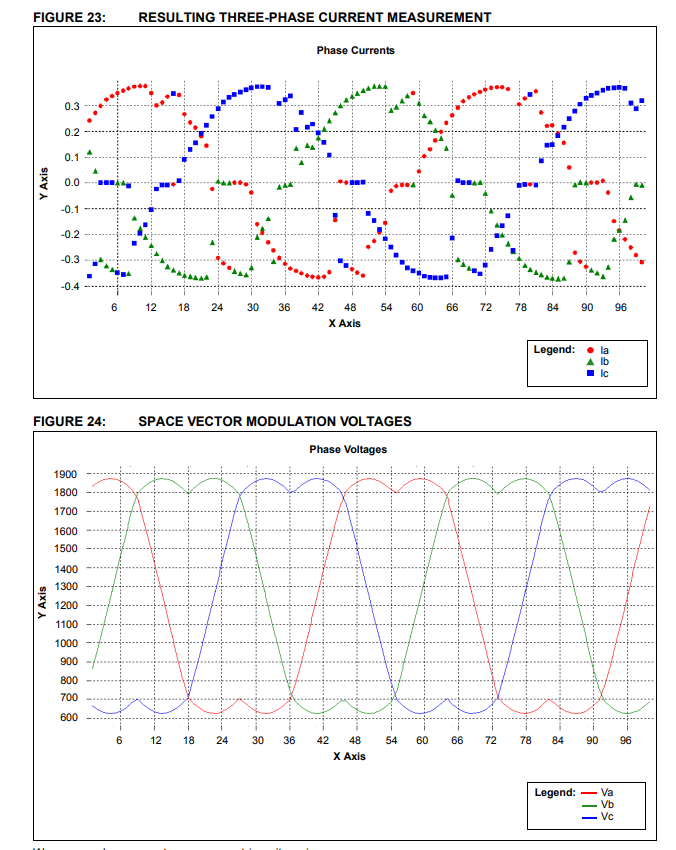
If current reconstruction is done without any
modification of the SVM pattern, that is, ignoring the
fact that during some periods current cannot be
reconstructed, the resulting three-phase current
measurement are shown in Figure 23. The SVM
voltages are shown in Figure 24.
ST 1 Shunt measurement method